|
Size: 504
Comment:
|
Size: 1147
Comment:
|
| Deletions are marked like this. | Additions are marked like this. |
| Line 17: | Line 17: |
| [[/ExampleCode]] | The PDF of an image can be calculated and displayed using the {{{pylab.hist}}} function or it can be calculated using the {{{scipy.histogram}}} function. === ASAR image of sea ice === {{attachment:seaice_intensity.png}} The received power (intensity) of a radar system is proportional to the normalized radar backscatter coefficient {{{#!latex $\sigma^0(f,\theta)$ }}} as a function of frequency and incidence angle. The backscatter coefficient describes how much of the transmitted energy is backscattered from the surface media. A (calibrated) ASAR image is made of the measured intensities ''I''. [[/ExampleCode|Source code and data]] |
Random variables
The measurements that form an image show statistical fluctuations. The image is characterised by a probability density function (PDF). The PDF f describes the probability of the occurrence of a discrete grey level q in the range of grey levels Q.
latex error! exitcode was 2 (signal 0), transscript follows:
Probability density functions and histograms
The PDF of an image can be calculated and displayed using the pylab.hist function or it can be calculated using the scipy.histogram function.
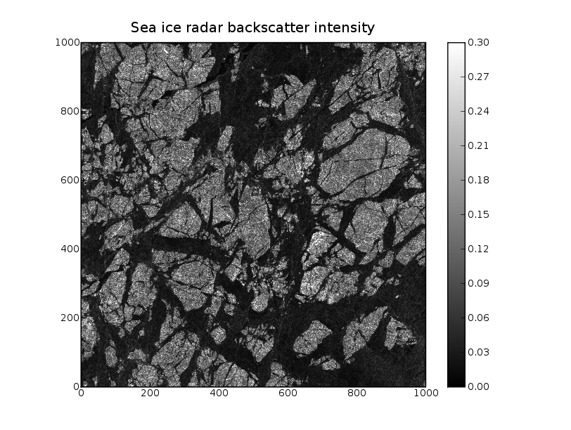
ASAR image of sea ice

The received power (intensity) of a radar system is proportional to the normalized radar backscatter coefficient
latex error! exitcode was 2 (signal 0), transscript follows:
as a function of frequency and incidence angle. The backscatter coefficient describes how much of the transmitted energy is backscattered from the surface media.
A (calibrated) ASAR image is made of the measured intensities I.
