Random variables
The measurements that form an image show statistical fluctuations. The image is characterised by a probability density function (PDF). The PDF f describes the probability of the occurrence of a discrete grey level q in the range of grey levels Q.
latex error! exitcode was 2 (signal 0), transscript follows:
Probability density functions and histograms
The PDF of an image can be calculated and displayed using the pylab.hist function or it can be calculated using the scipy.histogram function.
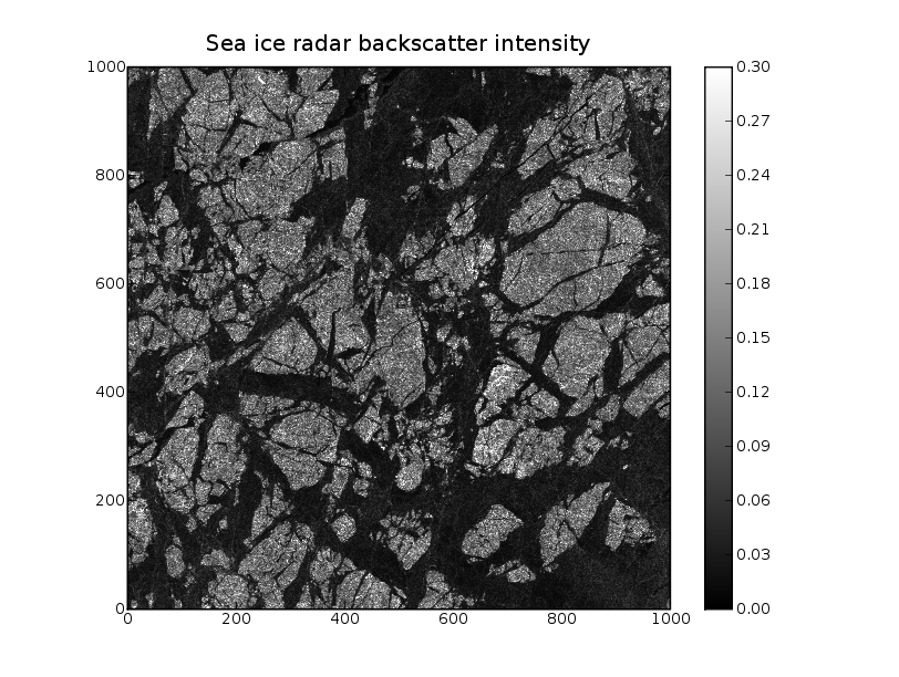
ASAR image of sea ice


The received power (intensity) of a radar system is proportional to the (normalized) radar backscatter coefficient
latex error! exitcode was 2 (signal 0), transscript follows:
as a function of frequency and incidence angle. The backscatter coefficient describes how much of the transmitted energy is backscattered from the surface media.
A (calibrated) ASAR image img(y,x)=I is made of the measured intensities I which can be directly related to the backscatter coefficient. A value of zero means that no energy is reflected from the surface whereas a value of one means the total reflection.
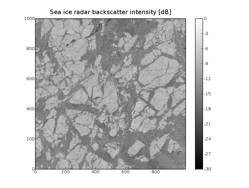
A useful representation of the intensity is the logarithmic transformation to the decibel unit
1 img_dB=10*log10(img)
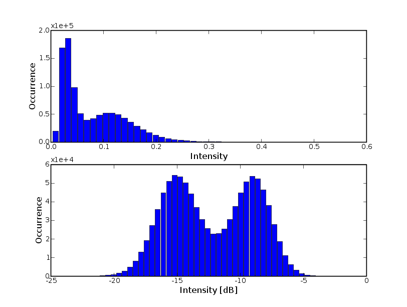
The PDF of the image above can be estimated from the number of occurrence of grey levels in the B intervals between q and q+dq and displayed using
1 hist(img,bins=50)
with the resolution B for 50 bins (intervals).

Estimation of the PDF parameters
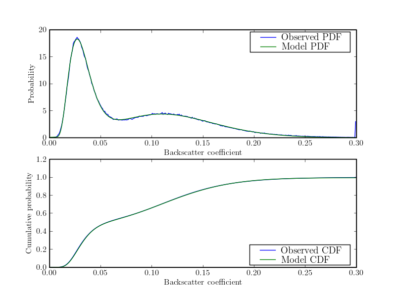
With assumptions about the statistical processes it is possible to model the probability distribution. In the following example it is assumed that the image is comprised of two surface types. The gamma distribution describes the statistical process that leads to the noise in radar images. A linear superposition of two gamma functions is used as a model for the PDF. A least square optimization is used with a cost/error function to estimate the model shape parameters (Line 9,11) and the linear superpostion coefficients (Line 14). The fitted model parameters p[6] and p[7] yield the fractions of the two surface types which are 47% and 53%, respectively

   1 from scipy import *
   2 from pylab import *
   3 import scipy.optimize as opti
   4 import scipy.stats as stats
   5
   6
   7 def my_pdf(p,x):
   8     """A linear mixture of two gamma PDF"""
   9     pdf1=stats.gamma.pdf(x,p[0],loc=p[1],scale=p[2])
  10     pdf2=stats.gamma.pdf(x,p[3],loc=p[4],scale=p[5])
  11     return pdf1*p[6]+pdf2*p[7]
  12
  13 def my_cdf(p,x):
  14     """A linear mixture of two gamma CDF"""
  15     cdf1=stats.gamma.cdf(x,p[0],loc=p[1],scale=p[2])
  16     cdf2=stats.gamma.cdf(x,p[3],loc=p[4],scale=p[5])
  17     return cdf1*p[6]+cdf2*p[7]
  18
  19 def my_cost(p,x,y):
  20     """The cost (error) function"""
  21     f=my_pdf(p,x)
  22     return y-f
  23
  24 #Read data
  25 img=reshape(fromfile('ASAR_seaice_mixed_20080421_f32_1000x1000.dat',dtype=float32),(1000,1000))
  26
  27 # Calculate relative frequency of occurence
  28 MIN,MAX,N=0.0,0.3,400
  29 h=histogram(img,bins=N,range=[MIN,MAX],normed=True)
  30 y,x=h[0],h[1]
  31 # Cumulative frequency (normalized)
  32 cdf=y.cumsum()*(MAX-MIN)/N
  33
  34 # Fit PDF model parameters to data by least squares optimization
  35 p0=[7.0,0.003,0.005,7.0,0.1,0.005,0.5,0.5 ] # initial guess
  36 p,success = opti.leastsq(my_cost, p0[:], args = (x, y))
  37
  38
  39 figure(1)
  40 subplot(2,1,1)
  41 plot(x,y)
  42 plot(x,my_pdf(p,x))
  43 legend(('Observed PDF','Model PDF'),'upper right')
  44 xlabel('Backscatter coefficient')
  45 ylabel('Probability')
  46 subplot(2,1,2)
  47 plot(x,cdf)
  48 plot(x,my_cdf(p,x))
  49 legend(('Observed CDF','Model CDF'),'lower right')
  50 xlabel('Backscatter coefficient')
  51 ylabel('Cumulative probability')
  52 savefig('model_stat.png',dpi=100)
  53 show()
