This page will be updated during the course 2015

Sea ice 2

Lecture, exercises and practical by Prof. Dr. Lars Kaleschke

Thursday 10:15-11:45
GB 5, Rm 006
Start 9. April

Description of the course

The lecture will cover the thermodynamic coupling between the sea ice, the ocean, and the atmosphere. It is designed for master-level students with moderate knowledge in numerical methods, scientific programming, and sea ice physics. A conceptual model of the Arctic will be derived and simulation results will be analyzed. For didactical reasons the model will be developed from scratch and kept as simple as possible, but complex enough to learn about the basic principles of the thermodynamic interaction between the ocean, the ice and the atmosphere for climatic, oceanographic and meteorological studies.

Links

Sea Ice Prediction Network Webinar 3 March 2015 by Elizabeth Hunke "Sea Ice Modeling: Characteristics and Processes Critical for the Radiation Budget"

Lesson 0 - A short introduction to the Python programming language

Lesson 1+2 - Ocean mixed layer and radiative forcing without sea ice and atmosphere

Lesson 1 - Simple ocean mixed layer.ipynb

Group results

/Group1 /Group2 /Group3 /Group4 /Group5 /Group6 /Group7 /Group8 /Group9 /Group10

Scenario 1

Ocean mixed layer forced by shortwave radiation only
No atmosphere
No exchange with deeper ocean layers, immediate mixing
Heat balance at the sea surface: Short wave incoming radiation + long wave outgoing radiation
$Q_{SW}^{\downarrow} + Q_{LW}^{\uparrow} = Q_{srf}$
Numerics: forward-in-time integration, finite differences
$\frac{\partial T_{ml}}{\partial t}\rho_w c_w h_{ml}=Q_{srf}$

Research questions

Compute the time evolution of the ocean mixed layer temperature T_ml(t) for different h_ml, initial temperatures T_ml(t=0), and short wave insolation Q_SW.

Estimate the typical time scale for stationarity and select appropriate time step delta_t for model integration.

Change insolation after the model has reached stationarity.

Lesson 3+4: Incoming shortwave radiation

Top of the atmosphere

A rough approximation for the flux of solar irradiance at the top of the atmosphere (TOA) can be derived from geometric considerations, e.g. Parkinson and Washington (1979)

$Q_{SW}^{\downarrow}=S \cos(Z)$

with the solar constant S=1360 W/m², the solar zenith angle Z. The cosine of the zenith angle is given by

$\cos Z=\sin \phi \sin \delta + \cos \phi \cos \delta \cos HA$

where

$\phi, \delta, HA,$

are latitude, declination, and hour angle in the equatorial coordinate system, respectively. The declination and hour angle are approximately calculated as

$\delta=23.44^\circ \times \cos (( 172- \textrm{day of year}) \times \pi/180) $$ $$ HA= (12 \textrm{hours - solar time}) \times \pi/12$

whereas the solar time is given in hours and it may be approximated by 24 hours per day.

Research questions

Calculate and plot the diurnal cycle of solar irradiance for the latitude of Hamburg on May 1st.
Calculate and plot the daily averaged solar irradiance for three latitudes (0, 50, 90) as a function of time
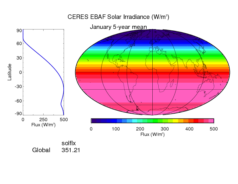
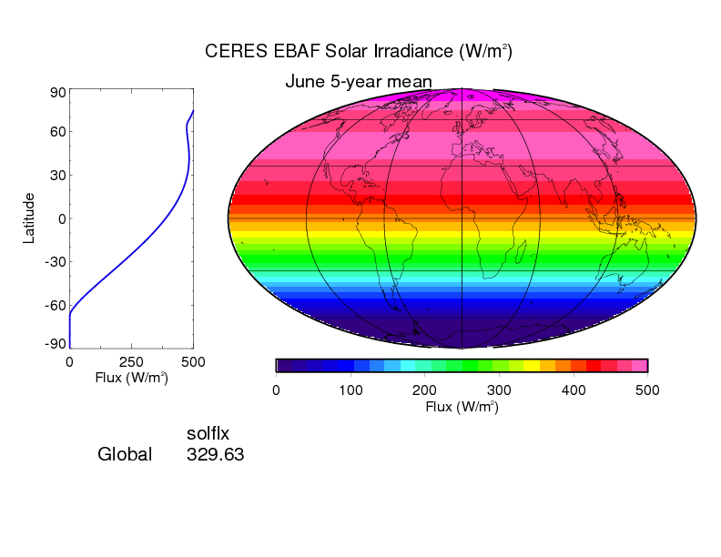
Calculate and plot the zonal averaged solar irradiance for different months (e.g. January and July)
Compare with the calculated irradiance with CERES measurements. See below for validation.
Calculate and plot the oceanic mixed layer temperature (h_ml=10m, T(0)=10^° C) forced with the solar irradiance (lat=60^°). Integration time shall be 3000 days. Explain the phase relation of temperature and irradiance.
Change the time step to one hour and calculate the diurnal cycle of the oceanic mixed layer temperature. Vary the mixed layer depth and latitude.
Add additional atmospheric longwave back radiation. Firstly, try a constant value of 100 W/m^2. Secondly, try Idso and Jackson's (1969) parameterization (see Parkinson, 1979). Modify the atmospheric temperature until the surface temperature is similar to a climatology.

Validation

Radiative flux measurements are available from the Clouds and the Earth s Radiant Energy System (CERES) sensor. Climatology products from the NASA Langley Research Center Atmospheric Science Data Center can be used to validate flux parameterizations. The CERES-Terra 5-year TOA global product has an easy to use browse interface. Select Terra based CERES EBAF (Net Adjusted) Browse Products (Monthly Means) Shortwave Incoming for a comparison to your results.

A long term numerical solution for the insolation quantities of the Earth (advanced)

For paleoclimate applications it is interesting to know how to calculate the insolation from astronomical parameters: La2004, source code

Lesson 5+6: Arctic surface energy balance

In this lesson we look at the energy fluxes at the ocean surface in polar latitudes. We will analyse the importance (magnitudes) of the different fluxes.

Scenario

Average climate at about 75-80 N
Ice growth model not yet included
Case 1: Ocean surface
Case 2: 100% sea ice cover
Energy fluxes based on empirical formulations given in Parkinson and Washington (1979)
Comparison to SHEBA data, and the forcing of Maykut and Untersteiner (1969) as used in Semtner (1976)

Research questions

Calculate and plot the daily/zonally averaged solar irradiance as a function of time (day of the year)
Modify the incoming shortwave radiation by a cloud factor (Eq. 4).
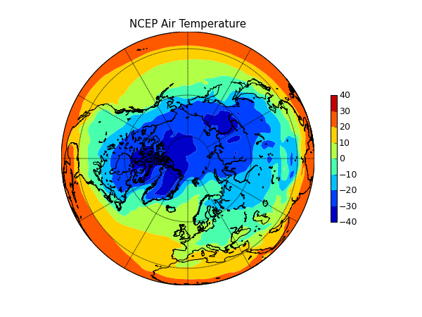
Calculate the incoming longwave radiation with Idso and Jackson's (1969) formula (Eq. 5). Take atmospheric temperature from climatolgy (e.g. NCEP file air.mon.ltm.nc) or SHEBA data (advanced)
Calculate the sensible heat flux as a function of different temperatures and wind speeds (sensitivity study, use NCEP wspd.mon.ltm.nc). This exercise can only be done when the ice model is ready (next session). We need the sea ice surface temperature which is calculated with the ice model. But for calculating the sensitivities one can simply assume constant sea ice surface temperatures.
Compare to observed fluxes, e.g. Huwald et al. 2005

Observed fluxes from SHEBA experiment

The Surface Heat Budget of the Arctic Ocean Project provides a unique data set for sea ice studies. Huwald et al. 2005 Table 2 Table with numbers only and columns ordered Jan. to Dec.

Table 2. Monthly and Yearly Means of the Energy Budget Components                                                                                                       

Var     Nov.    Dec.    Jan.    Feb.    March   April   May     June    July    Aug.    Sept.   Oct.    Year Mean
Fswd    0.1     0.0     0.0     5.1     46.3    142.3   248.7   280.4   211.4   110.8   39.9    20.0    92.1
Fswu    -0.1    0.0     0.0     -4.3    -39.4   -120.5  -204.4  -200.2  -135.9  -77.6   -25.9   -13.0   -68.5
Fsw     0.0     0.0     0.0     0.8     7.0     21.9    44.4    80.1    75.5    33.2    13.9    7.0     23.6
Fswp    0.0     0.0     0.0     0.1     0.6     1.8     3.6     9.6     12.8    5.5     0.5     0.2     2.9
Flwd    209.6   152.0   170.5   163.8   201.2   220.0   245.7   282.5   299.7   299.3   282.2   245.9   231.0
Flwu    -227.1  -185.2  -197.6  -190.2  -222.1  -242.4  -273.7  -308.2  -314.5  -310.7  -293.0  -260.1  -252.1
Flw     -17.6   -33.2   -27.1   -26.4   -20.8   -22.4   -28.0   -25.7   -14.8   -11.4   -10.7   -14.2   -21.0
Fsh     3.4     6.4     4.7     7.5     3.0     0.6     -1.1    1.5     1.6     -2.3    -0.4    1.5     2.4
Flh     0.3     0.3     0.1     0.0     -0.6    -0.5    -2.1    -2.2    -0.3    -1.5    -0.9    -0.3    -0.6
Fnet    -13.8   -26.5   -22.4   -18.2   -12.0   -2.1    11.9    44.2    49.1    12.5    3.8     -5.0    1.7
Fcs     14.8    19.7    13.1    13.1    8.3     7.0     2.2     -2.0    -3.7    -0.5    4.6     9.7     7.2
Fms     0.0     0.0     0.0     0.0     0.0     0.0     -3.2    -30.4   -48.0   -6.0    -4.0    -2.0    -7.8
Frs     1.0     -6.8    -9.3    -5.2    -3.7    4.8     10.9    12.4    -2.7    7.6     5.4     3.2     1.5
Fcb     -9.4    -13.0   -14.6   -13.3   -11.9   -8.2    -5.5    -2.6    -0.4    1.3     -2.3    -5.9    -7.1
Fmb     6.4     9.6     10.7    8.3     4.5     4.2     0.9     -7.3    -13.5   -15.2   -8.0    -0.8    0.0
Focn    3.0     3.4     3.9     5.0     7.4     4.0     4.6     9.9     13.9    13.9    10.3    6.7     7.1
Abbreviations are as follows: Fswd, Fswu, Fsw, Fswp, downward, upward, net, and penetrating shortwave radiation, respectively; Flwd, Flwu, Flw, downward, upward, and net longwave radiation, respectively; Fsh, Flh, sensible and latent heat flux, respectively; Fnet, net atmospheric heat fluxes; Fcs, conductive heat flux at the surface; Fms, energy of melt at the surface; Frs, net residual heat flux at the surface. The last three lines show the monthly and yearly means of the basal conductive heat flux (Fcb), energy of melt (Fmb), and the net residual heat flux, i.e., the ocean heat flux (Focn). All values are given in Wm-2.

How to use NCEP data

   1 from pylab import *
   2 from mpl_toolkits.basemap import Basemap, addcyclic
   3 #import scipy.io # Old Version
   4 from netCDF4 import Dataset
   5 
   6 filename='air.mon.ltm.nc'
   7 #fid=scipy.io.netcdf_file(filename,'r') # open file and create file identifier
   8 fid=Dataset(filename,'r',format='NETCDF4')
   9 
  10 print fid.description
  11 print 'File includes the following variables'
  12 for i in fid.variables.keys():
  13     print i
  14     
  15 lat0=fid.variables['lat']
  16 lon0=fid.variables['lon']
  17 air0=fid.variables['air']
  18 
  19 print 'Units of variable air ',air0.units
  20 
  21 # Make a copy for modification
  22 lon=lon0[:].copy()
  23 lat=lat0[:].copy()
  24 air=air0[:,:,:].copy()
  25 
  26 month=0 # select January
  27 
  28 T=air[month,:,:]
  29 
  30 # add cyclic for the gap between 360 and 0 deg longitude
  31 Tc, lonc = addcyclic(T, lon)
  32 
  33 m = Basemap(projection='ortho',lon_0=0.0,lat_0=90.0,resolution='l')
  34 x, y = m(*meshgrid(lonc,lat))
  35 ps=linspace(-40,40,9)
  36 m.contourf(x,y,Tc,ps,cmap=cm.jet)
  37 m.drawcoastlines()
  38 m.drawmeridians(arange(0, 360, 30))
  39 m.drawparallels(arange(-90, 90, 30))
  40 title('NCEP '+air0.var_desc)
  41 colorbar(shrink=0.5)
  42 savefig('ncep.png',dpi=75)
  43 show()

Lesson 7: Sea ice model

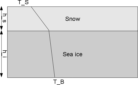
The 0-layer model of Semtner (1976) shall be implemented and tested. Use Newton-Raphson iteration (5 steps)

$x_{n+1}=x_n-f(x_n)/f'(x_n)$

to solve the energy balance equation for the surface temperature.

Standard parameters of Semtner (1976) in SI units:

$\begin{tabular}{llll} $k_i$ & thermal conductivity of sea ice & 2.0334 & W m$^{−1}$ K$^{−1}$ \\ $k_s$ & thermal conductivity of snow & 0.3096 & W m$^{−1}$ K$^{−1}$\\ $(\rho c)_i$ & volumetric heat capacity of sea ice & 1882.8 & kJ m$^{−3}$ K$^{−1}$\\ $(\rho c)_s$ & volumetric heat capacity of snow & 690.36 & kJ m$^{−3}$ K$^{−1}$\\ $(\rho c)_w$ & volumetric heat capacity of water & 4284 & kJ m$^{−3}$ K$^{−1}$\\ $L_B$ & volumetric heat of fusion of ice at lower surface & 2.67776 10$^5$ & kJ m$^{−3}$\\ $L_i$ & volumetric heat of fusion of ice at upper surface & 3.01248 10$^5$ & kJ m$^{−3}$\\ $L_s$ & volumetric heat of fusion of snow & 1.09621 10$^5$ & kJ m$^{−3}$\\ $\alpha_i$ & bare ice albedo & 0.64 & \\ $\alpha_s$ & snow albedo & 0.64-0.85 & \\ $I_0$ & fraction of penetrating shortwave radiation & 17 & \% \\ $\sigma$ & Stefan-Boltzmann constant (not correct!) & 5.7948 ·10$^{−8}$ & W m$^{−2}$ K$^{−4}$\\ $T_{f}$ & freezing temperature of sea water & -2 & $^\circ$C\\ \end{tabular}$

Scenario

Sea ice only, no snow, no ocean
Standard forcing (Table 1 in Semtner, 1976).

Research questions

Calculate and plot the time evolution of ice thickness
Discuss the influence of oceanic bottom heat flux

Deliverable: Report (15 August 2015)

Description of conducted experiments
Assumptions
Governing equations
Model variables
Forcing data
Model results (graph and descriptions)
Source code
Discussion and conclusions

Report format: PDF and .ipynb (if source code is not included in the PDF)

Send to: lars.kaleschke@uni-hamburg.de

Acknowledgments

This lecture is derived from content of a lecture Sea ice modeling by Aike Beckmann (Univ. Hamburg, Summer 2009) and a short course on Ice-Ocean Modeling and Data Assimilation which was conducted by Frank Kauker and Michael Karcher (Univ. Bremen, 6-7 December 2006).

Literature

References for download

Maykut, G.A. & N. Untersteiner, 1971: Some results from a time-dependent thermodynamic model of sea ice. J. Geophys. Res.,76, 1550-1575.

Semtner, A., 1976: A model for the thermodynamic growth of sea ice in numerical investigations of climate, J. Phys. Oceanogr, 6, 379-389.

Hibler III, W.D., 1979: A dynamic-thermodynamic sea ice model. J. Phys. Oceanogr., 9, 815-846.

Parkinson, C.L. & W.M. Washington, 1979: A large-scale numerical model of sea ice., J. Geophys. Res., 84, 311-337.

Sellers, W.D., 1969: A Global Climatic Model Based on the Energy Balance of the Earth-Atmosphere System, J. Appl. Met., 8(3), 392-400.

Philipp Johannes Griewank (2014): A 1D model study of brine dynamics in sea ice