Contents
Input/output and data formats
This lesson deals with the ways of reading and writing data in different formats
Basic Python
The file object can be used for reading and writing plain text as well as unformatted binary data. The following code writes a message in the file with the name out.txt, reads and print the data
write() writes a string to the file
read() reads complete file
read(N) reads N bytes
readlines() reads the file with linebreaks
readline() reads only the next line
Pickle
The pickle module implements an algorithm for serializing and de-serializing a Python object structure. Pickling is the process whereby a Python object hierarchy is converted into a byte stream, and unpickling is the inverse operation, whereby a byte stream is converted back into an object hierarchy. The cPickle module is a much faster implementation and should be preferred.
Comma Separated Values
The so-called CSV (Comma Separated Values) format is the most common import and export format for spreadsheets (Excel) and databases. The csv module enables CSV file reading and writing
NumPy/SciPy
Arrays can be read from a file and written to a file using the function and method:
fromfile(...)
.tofile(...)
HDF
NASA's standard file format, the http://hdf.ncsa.uiuc.edu/index.html is a self-describing data format. HDF files can contain binary data and allow direct access to parts of the file without first parsing the entire contents.
The HDF versions 4 and 5 are not compatible.
Different modules are available for reading and writing HDF files
HDF4 pyhdf
pyhdf is a python interface to the NCSA HDF4 library.
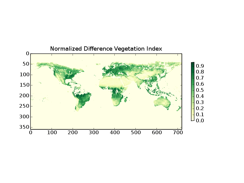
The following example demonstrates how to read level-3 data from the Multi-angle Imaging Spectral Radiometer (MISR) on the Terra Satellite
   1 from scipy import array
   2 from pylab import imshow,colorbar,title,savefig
   3 from pyhdf.SD import SD
   4
   5 f=SD('MISR_AM1_CGLS_MAY_2007_F04_0025.hdf')
   6 print f.datasets().keys()
   7 data=array(f.select('NDVI average').get())
   8 data[data<0]=0
   9
  10 imshow(data,interpolation='nearest',cmap=cm.YlGn)
  11 colorbar(shrink=0.5)
  12 title('Normalized Difference Vegetation Index')
Line 5 opens the HDF file object. line 6 prints the keywords of the included datasets. From this one can identify the keyword for the desired parameter. Line 7 reads the data in a SciPy array. Line 8 selects the negative (bad and missing) data and sets them to zero.

HDF5
PyTables is a package for managing hierarchical datasets and designed to efficiently and easily cope with extremely large amounts of data.
netCDF
PyNIO is a Python package that allows read and/or write access to a variety of data formats using an interface modelled on netCDF.
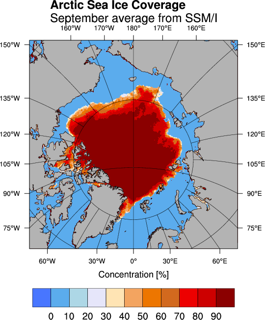
The following example demonstrates how to use the PyNGL module to read and display sea ice concentration data.
   1 import os
   2 from scipy import array,arange,nan
   3 from PyNGL import Ngl
   4 from PyNGL import Nio
   5
   6 def Ngl_map(C,lat,lon,psfile):
   7     rlist            = Ngl.Resources()
   8     rlist.wkColorMap = 'posneg_1'
   9     wks_type = "ps"
  10     wks = Ngl.open_wks(wks_type,psfile,rlist)
  11     resources = Ngl.Resources()
  12     resources.sfXArray        = lon[:,:]
  13     resources.sfYArray        = lat[:,:]
  14     resources.mpProjection          = "Stereographic"
  15     resources.mpDataBaseVersion     = "MediumRes"
  16     resources.mpLimitMode           = "LatLon"
  17     resources.mpMinLonF             = 0
  18     resources.mpMaxLonF             = 360
  19     resources.mpMinLatF             = 65
  20     resources.mpMaxLatF             = 90
  21     resources.mpCenterLonF           = 0.
  22     resources.mpFillOn     = True
  23     igray = Ngl.new_color(wks,0.7,0.7,0.7)
  24     resources.mpFillColors = [0,-1,igray,-1]
  25     resources.cnLineDrawOrder      = "Predraw"
  26     resources.cnFillOn             = True
  27     resources.cnFillDrawOrder       = "Predraw"
  28     resources.cnLineLabelsOn        = False
  29     resources.nglSpreadColorStart  = 8
  30     resources.nglSpreadColorEnd      = -2
  31     resources.cnLevelSelectionMode = "ExplicitLevels" # Define own levels.
  32     resources.cnLevels             = arange(0.,100,10)
  33     resources.lbTitleString             = 'Concentration [%]'
  34     resources.lbOrientation             = "Horizontal"
  35     resources.cnFillMode           = "RasterFill"
  36     resources.cnLinesOn            = False
  37     resources.tiMainString     = "~F22~Arctic Sea Ice Coverage~C~~F21~September average from SSM/I"
  38     map = Ngl.contour_map(wks,C[:,:],resources)
  39
  40 grid = Nio.open_file('grid_north_12km.nc')
  41 lat=array(grid.variables['latitude'])
  42 lon=array(grid.variables['longitude'])
  43 nc = Nio.open_file('climatology_09.nc')
  44 C=array(nc.variables['concentration'])[0,:,:].astype(float)
  45 Ngl_map(C,lat,lon,'map')
  46 os.system('gv map.ps &')
The data files can be downloaded from the ftp server of the Center for Satellite Exploitation and Research (CERSAT) which is one of the major world data centers for oceanography.
The September mean sea ice concentration values derived from the Special Sensor Microwave Imager (SSM/I) are stored in the netCDF file climatology_09.nc . Compressed data with the extension .Z or .gz can be uncompressed using uncompress or gunzip, respectively. A description of the data and the algorithm can be found here.
The main program that reads the data starts in line 40. At first the coordinates of the corresponding pixels are read into the variables lat and lon. The ice concentration data are read in the variable C. The function Ngl_map creates a postscript output in the file map.ps which is displayed using the command gv.

Various Satellite data formats
The Geospatial Data Abstraction Library (GDAL) has a single abstract data model for all supported formats
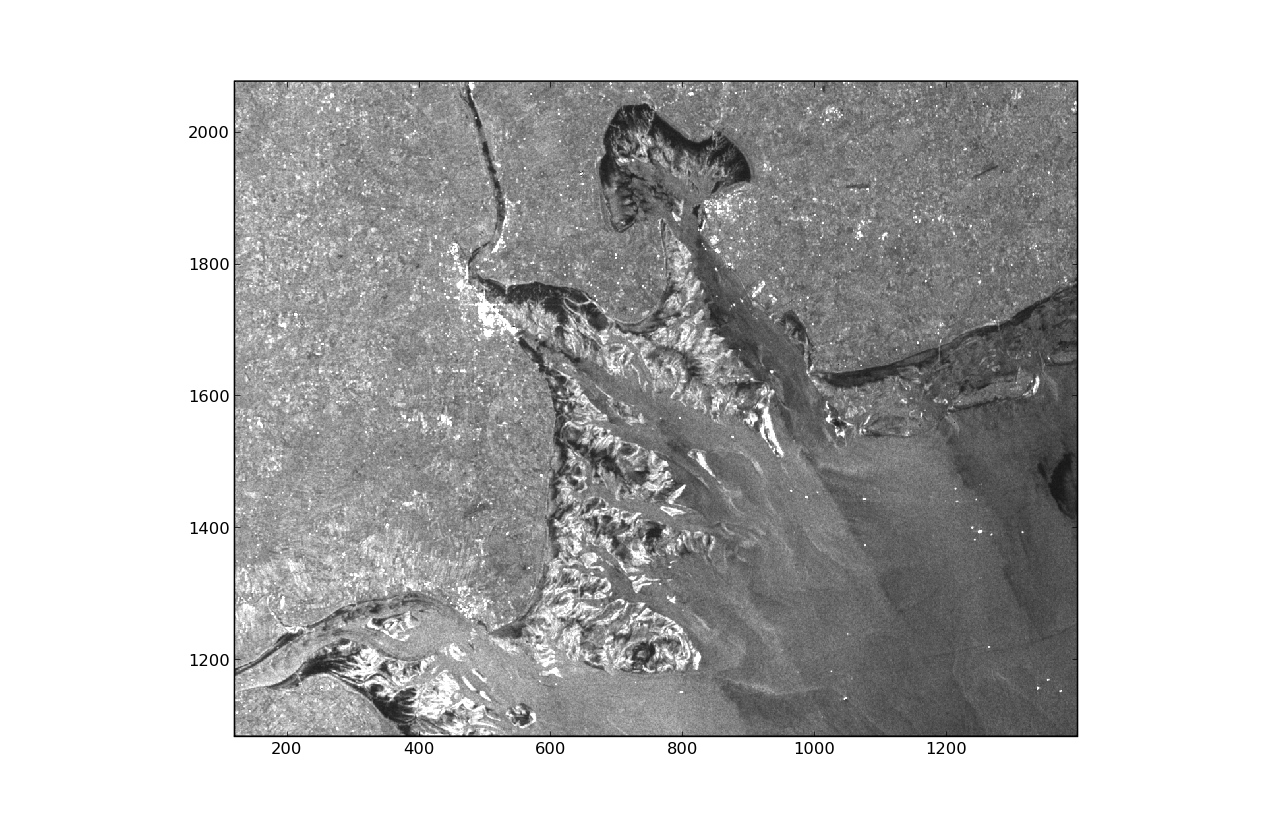
The following code demonstrates how to read in an Envisat ASAR image using the gdal module.
   1 import gdal, struct
   2 from scipy import array,empty,uint16
   3 from pylab import imshow
   4
   5 filename='/pf/u/u242023/ASA_IMM_1PNPDK20080410_095538_000001462067_00337_31954_4832.N1'
   6
   7 f=gdal.Open(filename)
   8 a=f.GetRasterBand(1)
   9 img=empty((a.YSize,a.XSize),dtype=uint16)
  10
  11
  12 for yi in xrange(a.YSize):
  13     scanline=struct.unpack("H"*a.XSize,a.ReadRaster(0,yi,a.XSize,1,a.XSize,1,gdal.GDT_UInt16))
  14     img[yi,:]=array(scanline).astype(uint16)
  15
  16 imshow(img,vmin=0,vmax=3000,interpolation='nearest',origin='lower')
