Sea ice 2

Lecture, exercises and practical by Jun.-Prof. Dr. Lars Kaleschke

• Monday 13:30-15:00
• Room ZMAW 022

Description of the course

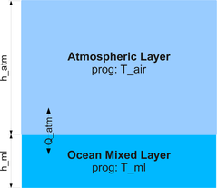
The lecture will cover the thermodynamic coupling between the sea ice, the ocean, and the atmosphere. It is designed for master-level students with moderate knowledge in numerical methods, scientific programming, and sea ice physics. A conceptual model of the Arctic will be derived and simulation results will be analyzed. For didactical reasons the model will be developed from scratch and kept as simple as possible, but complex enough to learn about the basic principles of the thermodynamic interaction between the ocean, the ice and the atmosphere for climatic, oceanographic and meteorological studies.

Deliverable: Report (15 August 2010)

• Description of conducted experiments
• Assumptions
• Governing equations
• Model variables
• Forcing data
• Model results (graph and descriptions)
• Source code
• Discussion and conclusions

Acknowledgments

This lecture is based on content taken from a lecture Sea ice modeling by Aike Beckmann (Univ. Hamburg, Summer 2009) and a short course on Ice-Ocean Modeling and Data Assimilation which was conducted by Frank Kauker and Michael Karcher (Univ. Bremen, 6-7 December 2006).

Project work: source code, results

/Gruppe1 /Gruppe2 /Gruppe3 /Gruppe4 /Gruppe5

Table of Contents

Lesson 1+2 - Ocean mixed layer and radiative forcing without sea ice and atmosphere

Scenario 1

• Ocean mixed layer forced by shortwave radiation only
• No atmosphere
• No exchange with deeper ocean layers, immediate mixing
• Heat balance at the sea surface: Short wave incoming radiation + long wave outgoing radiation

  latex error! exitcode was 2 (signal 0), transscript follows:
  
  

• Numerics: forward-in-time integration, finite differences

• latex error! exitcode was 2 (signal 0), transscript follows:
  
  

Research questions

Compute the time evolution of the ocean mixed layer temperature T_ml(t) for different h_ml, initial temperatures T_ml(t=0), and short wave insolation Q_SW.

Estimate the typical time scale for stationarity and select appropriate time step delta_t for model integration.

Change insolation after the model has reached stationarity.

Lesson 3+4+5: Incoming shortwave radiation

Top of the atmosphere

A rough approximation for the flux of solar irradiance at the top of the atmosphere (TOA) can be derived from geometric considerations

latex error! exitcode was 2 (signal 0), transscript follows:

with the solar constant S=1360 W/m², the solar zenith angle Z. The cosine of the zenith angle is given by

latex error! exitcode was 2 (signal 0), transscript follows:

where

latex error! exitcode was 2 (signal 0), transscript follows:

are latitude, declination, and hour angle, respectively. The declination and hour angle are calculated as

latex error! exitcode was 2 (signal 0), transscript follows:

Research questions

• Calculate and plot the diurnal cycle of solar irradiance for the latitude of Hamburg on April 19.
• Calculate and plot the daily averaged solar irradiance for three latitudes (0, 50, 90) as a function of time
• Calculate and plot the zonal averaged solar irradiance for different months (e.g. January and July)
• Compare with the calculated irradiance with CERES measurements

• Calculate and plot the oceanic mixed layer temperature (h_ml=30m, T(0)=10^° C) forced with the solar irradiance (lat=30^°). Integration time shall be 3000 days. Explain the relation of temperature and irradiance.

• Change the time step to one hour and calculate the diurnal cycle of the oceanic mixed layer temperature. Vary the mixed layer depth and latitude.

Validation

Radiative flux measurements are available from the Clouds and the Earth s Radiant Energy System (CERES) sensor. Climatology products from the NASA Langley Research Center Atmospheric Science Data Center can be used to validate flux parameterizations. The CERES-Terra 5-year TOA global product has an easy to use browse interface.

Lesson 5+6: Energy fluxes at the ocean surface

In this lesson we look at the energy fluxes at the ocean surface in polar latitudes. We will analyse the importance (magnitudes) of the different fluxes.

Scenario

• (Ocean) surface kept constant at the freezing point or at the air temperature

• Prescribed atmospheric temperature, as a first try with a constant first guess, secondly with numbers from climatolgy (e.g. NCEP)

• Energy fluxes based on empirical formulations given in Parkinson and Washington (1979)
• Incoming short wave radiation + incoming and outgoing long wave radiation + sensible heat fluxes
• Zonal average 65N-90N

Research questions

• Calculate and plot the daily and zonally averaged solar irradiance as a function of time (day of the year)
• Modify the irradiance by a cloud factor [Laevastu, 1960].
• Calculate the incoming longwave radiation with Idso and Jackson's (1969) formula.
• Calculate the sensible heat flux as a function of typical temperature differences and wind speed

• Compare to observed fluxes, e.g. Huwald et al. 2005

Observed fluxes from SHEBA experiment

The Surface Heat Budget of the Arctic Ocean Project provides a unique data set for sea ice studies.

Huwald et al. 2005 Table 2 Table with numbers only and columns ordered Jan. to Dec.

Table 2. Monthly and Yearly Means of the Energy Budget Componentsa                                                                                                      

Var     Nov.    Dec.    Jan.    Feb.    March   April   May     June    July    Aug.    Sept.   Oct.    Year Mean
Fswd    0.1     0.0     0.0     5.1     46.3    142.3   248.7   280.4   211.4   110.8   39.9    20.0    92.1
Fswu    -0.1    0.0     0.0     -4.3    -39.4   -120.5  -204.4  -200.2  -135.9  -77.6   -25.9   -13.0   -68.5
Fsw     0.0     0.0     0.0     0.8     7.0     21.9    44.4    80.1    75.5    33.2    13.9    7.0     23.6
Fswp    0.0     0.0     0.0     0.1     0.6     1.8     3.6     9.6     12.8    5.5     0.5     0.2     2.9
Flwd    209.6   152.0   170.5   163.8   201.2   220.0   245.7   282.5   299.7   299.3   282.2   245.9   231.0
Flwu    -227.1  -185.2  -197.6  -190.2  -222.1  -242.4  -273.7  -308.2  -314.5  -310.7  -293.0  -260.1  -252.1
Flw     -17.6   -33.2   -27.1   -26.4   -20.8   -22.4   -28.0   -25.7   -14.8   -11.4   -10.7   -14.2   -21.0
Fsh     3.4     6.4     4.7     7.5     3.0     0.6     -1.1    1.5     1.6     -2.3    -0.4    1.5     2.4
Flh     0.3     0.3     0.1     0.0     -0.6    -0.5    -2.1    -2.2    -0.3    -1.5    -0.9    -0.3    -0.6
Fnet    -13.8   -26.5   -22.4   -18.2   -12.0   -2.1    11.9    44.2    49.1    12.5    3.8     -5.0    1.7
Fcs     14.8    19.7    13.1    13.1    8.3     7.0     2.2     -2.0    -3.7    -0.5    4.6     9.7     7.2
Fms     0.0     0.0     0.0     0.0     0.0     0.0     -3.2    -30.4   -48.0   -6.0    -4.0    -2.0    -7.8
Frs     1.0     -6.8    -9.3    -5.2    -3.7    4.8     10.9    12.4    -2.7    7.6     5.4     3.2     1.5
Fcb     -9.4    -13.0   -14.6   -13.3   -11.9   -8.2    -5.5    -2.6    -0.4    1.3     -2.3    -5.9    -7.1
Fmb     6.4     9.6     10.7    8.3     4.5     4.2     0.9     -7.3    -13.5   -15.2   -8.0    -0.8    0.0
Focn    3.0     3.4     3.9     5.0     7.4     4.0     4.6     9.9     13.9    13.9    10.3    6.7     7.1
Abbreviations are as follows: Fswd, Fswu, Fsw, Fswp, downward, upward, net, and penetrating shortwave radiation, respectively; Flwd, Flwu, Flw, downward, upward, and net longwave radiation, respectively; Fsh, Flh, sensible and latent heat flux, respectively; Fnet, net atmospheric heat fluxes; Fcs, conductive heat flux at the surface; Fms, energy of melt at the surface; Frs, net residual heat flux at the surface. The last three lines show the monthly and yearly means of the basal conductive heat flux (Fcb), energy of melt (Fmb), and the net residual heat flux, i.e., the ocean heat flux (Focn). All values are given in Wm-2.                                                                                                   

Lesson 7: Sea ice model

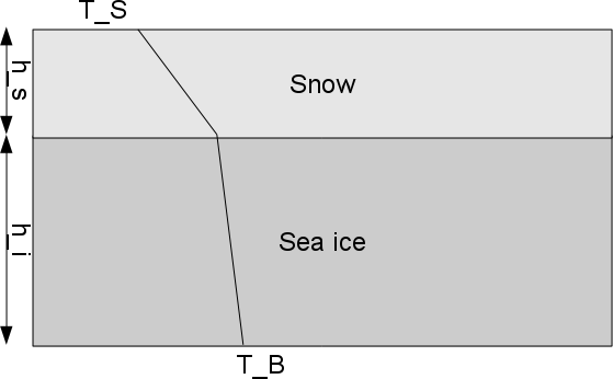
The 0-layer model of Semtner (1976) shall be implemented and tested.

Standard parameters of Semtner (1976) in SI units:

latex error! exitcode was 2 (signal 0), transscript follows:

Scenario

• Sea ice only, no snow, no ocean
• Standard forcing (Table 1 in Semtner, 1976).

Research questions

• Calculate and plot the time evolution of ice thickness

Literature

References for download

Maykut, G.A. & N. Untersteiner, 1971: Some results from a time-dependent thermodynamic model of sea ice. J. Geophys. Res.,76, 1550-1575.

Semtner, A., 1976: A model for the thermodynamic growth of sea ice in numerical investigations of climate, J. Phys. Oceanogr, 6, 379-389.

Hibler III, W.D., 1979: A dynamic-thermodynamic sea ice model. J. Phys. Oceanogr., 9, 815-846.

Parkinson, C.L. & W.M. Washington, 1979: A large-scale numerical model of sea ice., J. Geophys. Res., 84, 311-337.

Sellers, W.D., 1969: A Global Climatic Model Based on the Energy Balance of the Earth-Atmosphere System, J. Appl. Met., 8(3), 392-400.