|
Size: 719
Comment:
|
← Revision 7 as of 2008-12-08 13:15:56 ⇥
Size: 1323
Comment:
|
| Deletions are marked like this. | Additions are marked like this. |
| Line 7: | Line 7: |
| = Random variables = | = Image statistics = |
| Line 9: | Line 9: |
| The measurements that form an image show statistical fluctuations. The image is characterised by a probability density function (PDF). The PDF ''f'' describes the probability of the occurrence of a discrete grey level ''q'' in the range of grey levels ''Q''. | |
| Line 11: | Line 10: |
| {{{#!latex $\sum_{q=1}^Qf_q=1$ |
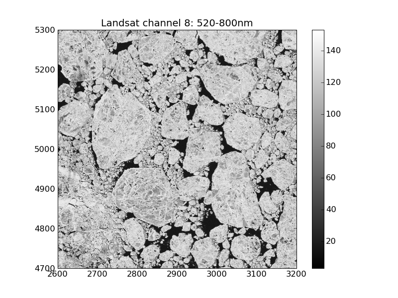
The image is characterised by a '''probability density function''' (PDF). The PDF describes the probability of the occurrence of the discrete grey levels. == Example == {{attachment:landsat_b80.png}} The following code calculates the PDF {{{pdf(q)}}} for a ''byte'' image {{{img}}} in the intervall {{{[0,255]}}} {{{#!python h=histogram(img,bins=256,range=[0,255],normed=True) pdf,x=h[0],h[1] |
| Line 15: | Line 24: |
| == Probability density functions and histograms == | The expression {{{normed=True}}} is used for the normalization of the PDF. {{{#!latex $\sum_{q=0}^{255}pdf(q)=1$ }}} |
| Line 17: | Line 29: |
| The PDF of an image can be calculated and displayed using the {{{pylab.hist}}} function or it can be calculated using the {{{scipy.histogram}}} function. |
The anti-derivative of the PDF is the '''cumulative density function''' (CDF). {{{#!latex $cdf(q)=\sum_{q'=0}^{q}pdf(q')$ }}} |
| Line 20: | Line 34: |
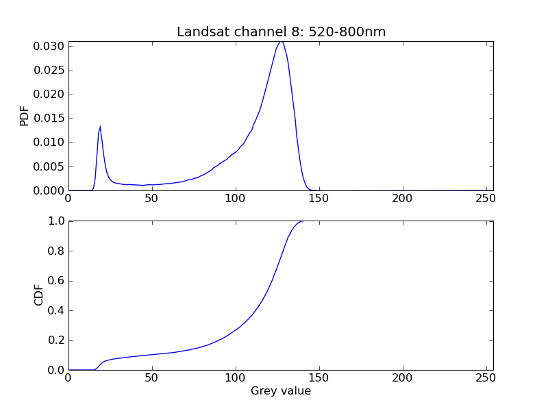
| [[attachment:landsat_b80.png]] | The cumulative sum can be calculated using {{{#!python cdf=pdf.cumsum() }}} {{attachment:landsat_b80_pdfcdf.png}} The probability of the occurence of grey levels in the interval {{{[a,b]}}} can be calculated from the CDF. In the example shown, the probability of grey levels to occur in the interval {{{[12,25]}}} according to the first peak is 0.068. So roughly 7% of the image pixels are in this grey level interval. {{{#!python cdf[25]-cdf[12] 0.068 }}} |
Image statistics
The image is characterised by a probability density function (PDF). The PDF describes the probability of the occurrence of the discrete grey levels.
Example

The following code calculates the PDF pdf(q) for a byte image img in the intervall [0,255]
The expression normed=True is used for the normalization of the PDF.
latex error! exitcode was 2 (signal 0), transscript follows:
The anti-derivative of the PDF is the cumulative density function (CDF).
latex error! exitcode was 2 (signal 0), transscript follows:
The cumulative sum can be calculated using
1 cdf=pdf.cumsum()

The probability of the occurence of grey levels in the interval [a,b] can be calculated from the CDF. In the example shown, the probability of grey levels to occur in the interval [12,25] according to the first peak is 0.068. So roughly 7% of the image pixels are in this grey level interval.
