|
Size: 2978
Comment:
|
Size: 3640
Comment:
|
| Deletions are marked like this. | Additions are marked like this. |
| Line 17: | Line 17: |
| * Read (copy) a variable to an array {{{a=fid.variables['NAME'][:].copy()}}} | * Read (copy) a variable to an array {{{a=fid.variables[NAME][:].copy()}}} |
| Line 19: | Line 19: |
== Attributes == After opening a NetCDF file you can examine the variable NAME (string) {{{#!python var=fid.variables[NAME] }}} by looking at their methods, e.g. {{{var.attributes}}} or {{{var.dimension}}}. |
|
| Line 26: | Line 34: |
| = Excercise = | = Excercise 1 = |
| Line 28: | Line 36: |
| Write scripts | Download NCEP/NCAR reanalysis atmospheric surface temperature monthly mean values. Examine the variables and their attributes. * What are their dimensions? * What is the meaning of the dimensions? * What are the units? * What are the scaling? * How are the missing values marked? * Select the grid cell for the position of Hamburg and plot the temperature time series. = Excercise 2 = Write scripts (or try to understand the code below) |
NetCDF
You can use the scipy.io subroutines to read NetCDF data:
Open a file with fid=scipy.io.netcdf_file(filename,'r')
Print variables with fid.variables.keys()
Read (copy) a variable to an array a=fid.variables[NAME][:].copy()
Close the file fid.close()
Attributes
After opening a NetCDF file you can examine the variable NAME (string)
1 var=fid.variables[NAME]
by looking at their methods, e.g. var.attributes or var.dimension.
NetCDF Data Examples
ftp://ftp.ifremer.fr/ifremer/cersat/products/gridded/psi-concentration/data/ Sea ice
http://www.esrl.noaa.gov/psd/data/reanalysis/reanalysis.shtml NCEP/NCAR Atmopsheric Reanalysis
Excercise 1
Download NCEP/NCAR reanalysis atmospheric surface temperature monthly mean values. Examine the variables and their attributes.
- What are their dimensions?
- What is the meaning of the dimensions?
- What are the units?
- What are the scaling?
- How are the missing values marked?
- Select the grid cell for the position of Hamburg and plot the temperature time series.
Excercise 2
Write scripts (or try to understand the code below)
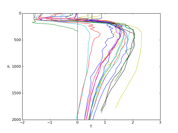
to download all Argo data in the Atlantic for the last month, and
- to plot the pressure against the temperature for only those profiles with a surface temperature below -1 deg C.
   1 #download_argo.py
   2 import os,os.path
   3 from ftplib import FTP
   4
   5 tmp_dir='/home/lars/data/tmp/'
   6 ftp_adr='ftp.ifremer.fr'
   7 ftp_dir='/ifremer/argo/geo/atlantic_ocean/2009/11/'
   8
   9 ftp = FTP(ftp_adr)   # connect to host, default port
  10 ftp.login()          # user anonymous, passwd anonymous@
  11 ftp.cwd(ftp_dir)
  12
  13 file_list=ftp.nlst()
  14
  15 for f in file_list:
  16     urlfile='ftp://'+ftp_adr+ftp_dir+f
  17     localfile=tmp_dir+f
  18
  19     if not(os.path.exists(localfile)):
  20         print 'Getting file '+f
  21          #We use curl instead of ftp.retrbinary for download
  22         os.system("curl -s -k -o "+localfile+"  "+urlfile)
  23     else:
  24         print 'file '+f+' exists'
  25
  26 ftp.close()
   1 #Plot Argo profiles with surface temperature below 1 deg C
   2 import scipy.io as io
   3 import glob
   4 from pylab import *
   5
   6 tmp_dir='/home/lars/data/tmp/'
   7 file_liste=glob.glob(tmp_dir+'*.nc')
   8
   9 D={}# Empty dictionary to store selected profiles
  10 for f in file_liste:
  11     print f
  12
  13     # Open netcdf data file
  14     fid=io.netcdf_file(f,'r')
  15
  16     #print fid.variables.keys()
  17
  18     # Make a copy of the content
  19     lat=fid.variables['LATITUDE'][:].copy()
  20     lon=fid.variables['LONGITUDE'][:].copy()
  21     T=fid.variables['TEMP'][:].copy()
  22     P=fid.variables['PRES'][:].copy()
  23
  24     T[T>=99999]=nan # Set 99999.0 to "Not a Number"
  25     P[P>=99999]=nan
  26
  27     (nr_profs,Z)=T.shape # Get dimension
  28
  29     for i in range(nr_profs):
  30         if T[i,0]<1.0: # Select only those profiles with surface temperature below 1 deg C
  31             # Store profile in dictionary with the position as a key
  32             D[(lat[i],lon[i])]=(T[i,:],P[i,:])
  33     # Close data file
  34     fid.close()
  35
  36
  37 # Plot data
  38 figure()
  39 for k in D.keys():
  40     print k
  41     plot(D[k][0][:],D[k][1][:])
  42 axis([-2,3,2000,0])
  43 xlabel('T')
  44 ylabel('P')
  45 show()

