|
Size: 1921
Comment:
|
Size: 3878
Comment:
|
| Deletions are marked like this. | Additions are marked like this. |
| Line 36: | Line 36: |
| {{{ Help on function griddata in module matplotlib.mlab: griddata(x, y, z, xi, yi) ``zi = griddata(x,y,z,xi,yi)`` fits a surface of the form *z* = *f*(*x*, *y*) to the data in the (usually) nonuniformly spaced vectors (*x*, *y*, *z*). :func:`griddata` interpolates this surface at the points specified by (*xi*, *yi*) to produce *zi*. *xi* and *yi* must describe a regular grid, can be either 1D or 2D, but must be monotonically increasing. A masked array is returned if any grid points are outside convex hull defined by input data (no extrapolation is done). Uses natural neighbor interpolation based on Delaunay triangulation... }}} |
|
| Line 41: | Line 59: |
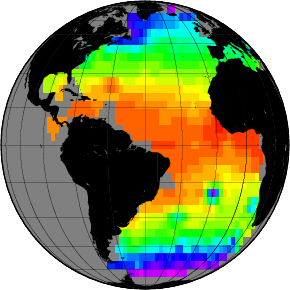
| Nearest neighbor gridding with 5 degree grid cell size {{{nearneighbor lat_lon_T.tab -Rd -I300m -S300m -N1 -Ggrid.nc}}} |
[[http://gmt.soest.hawaii.edu/gmt/doc/gmt/html/GMT_Tutorial/node44.html|Nearest neighbor gridding]] with 5 degree grid cell size {{{ nearneighbor lat_lon_T.tab -Rd -I300m -S300m -N1 -Ggrid.nc }}} |
| Line 50: | Line 69: |
| Plot grid files in 2-D | |
| Line 51: | Line 71: |
| grdimage grid.nc -Rg -JG-45/0/4i -Cg.cpt -K > out.ps | grdimage grid.nc -Rd -JG-45/0/4i -Cg.cpt -K > out.ps |
| Line 54: | Line 74: |
| Plot continents on map | |
| Line 58: | Line 79: |
| Show resulting postscript map | |
| Line 62: | Line 84: |
| Convert to png format for this Wiki page {{{ convert -trim out.ps out.png }}} Common options: {{{ -R specifies the min/max coordinates of data region in user units. -J Selects map projection. -K Means allow for more plot code to be appended later. -O means Overlay plot mode. }}} |
|
| Line 63: | Line 100: |
=== Exercises === Read the GMT manual: * Find out the meaning of the options I, S, N of the nearest neighbor gridding * What does -Rd mean? * What projection was chosen? Produce new plots: * Select a sub region of the data, i.e. only the North Atlantic. * Select a different projection * Plot the data with this projection Use new interpolation parameters: * Modify grid cell size (increment) to obtain a finer grid * Modify search radius Interaction with Python: * Read the GMT-netcdf file into Python with {{{scipy.io.netcdf_file}}}, (variable z) * Write a Python script that does the interpolation with GMT by using {{{os.system()}}} Use different interpolation technique: * {{{surface}}}, adjustable tension continuous curvature surface gridding algorithm |
Contents
2-dimensional interpolation and gridding
2-dimensional interpolation and gridding is a common problem for the representation of measurements on a map. Usually measurements are taken at irregular sample points and not in a regular grid. There are various approaches for the problem and the best solution depends on the data.
In the following we will look at oceanographic parameters that have been measured with the Argo system.
Example data from Argo system
Data are provided at, i.e. ftp://ftp.ifremer.fr//ifremer/argo/
First we have to download the data. Here is a /download script that can be used to retrieve one month of Argo data.
We extract only the surface temperature to reduce the large amount of data. This /extract script generates an overview of the data and writes the surface temperature in a file lat_lon_T.tab which contains latitude, longitude and surface temperature. We can use this file in the following.

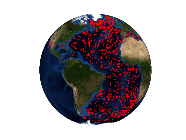
Argo positions of measurements

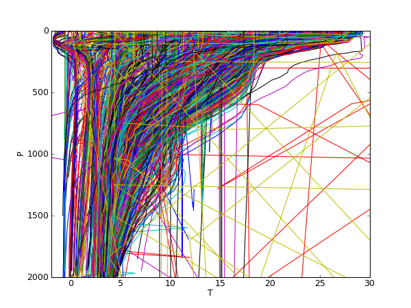
Measured temperature profiles (unfiltered data).
Tools for 2-dimensional interpolation and gridding
Python
Help on function griddata in module matplotlib.mlab:

griddata(x, y, z, xi, yi)
    ``zi = griddata(x,y,z,xi,yi)`` fits a surface of the form *z* =
    *f*(*x*, *y*) to the data in the (usually) nonuniformly spaced
    vectors (*x*, *y*, *z*).  :func:`griddata` interpolates this
    surface at the points specified by (*xi*, *yi*) to produce
    *zi*. *xi* and *yi* must describe a regular grid, can be either 1D
    or 2D, but must be monotonically increasing.

    A masked array is returned if any grid points are outside convex
    hull defined by input data (no extrapolation is done).

    Uses natural neighbor interpolation based on Delaunay
    triangulation...
GMT
Nearest neighbor gridding with 5 degree grid cell size
nearneighbor lat_lon_T.tab -Rd -I300m -S300m -N1 -Ggrid.nc
Generate color table:
makecpt -Crainbow -T-2/30/1 > g.cpt
Plot grid files in 2-D
grdimage grid.nc -Rd -JG-45/0/4i -Cg.cpt -K > out.ps
Plot continents on map
pscoast -Rd -JG-45/0/4i -B15g15 -Dc -Gblack -P -O >> out.ps
Show resulting postscript map
gv out.ps
Convert to png format for this Wiki page
convert -trim out.ps out.png
Common options:
-R specifies the min/max coordinates of data region in user units.
-J Selects map projection.
-K Means allow for more plot code to be appended later.
-O means Overlay plot mode.

Exercises
Read the GMT manual:
- Find out the meaning of the options I, S, N of the nearest neighbor gridding
- What does -Rd mean?
- What projection was chosen?
Produce new plots:
- Select a sub region of the data, i.e. only the North Atlantic.
- Select a different projection
- Plot the data with this projection
Use new interpolation parameters:
- Modify grid cell size (increment) to obtain a finer grid
- Modify search radius
Interaction with Python:
Read the GMT-netcdf file into Python with scipy.io.netcdf_file, (variable z)
Write a Python script that does the interpolation with GMT by using os.system()
Use different interpolation technique:
surface, adjustable tension continuous curvature surface gridding algorithm
